Mathematical details of the logistic equation are explained, and
applied to Australia's population projections....
Let P(t) represent the population of a species at time t.
If growth is to end, the time rate of change of the population
must fall to zero. The objective function is thus:
dP/dt = 0 ...(1)
We don't know what sort of function to use for dP/dt. Alfred Lotka
postulated that it might be some function of the population size:
dP/dt = f(P) = 0 ...(2)
The Taylor series expansion of any function f(P) gives:
dP/dt = bP + dP2 + gP3 + .... ...(3)
Using one term of the taylor series expansion for f(P) gives an
exponentially increasing population - and can't satisfy the
objective (1).
Taking the first two terms of the taylor series expansion is the
simplest approximation to f(P) that will permit a non-trivial
solution to (1).
dP/dt = bP + dP2 ...(4)
Solving (1) and (4) gives
0 = Plimit ( b + dPlimit )
hence
b + dPlimit= 0

 Plimit = - b /d                     ...(4a)

(
Since

 Plimit ≥ 0

 we would expect that b  ≥ 0 and d ≤ 0  in equation (4).
 )
|
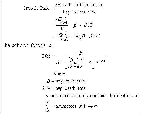
The growth rate of the population is defined as the growth in
the population, divided by the size of the population. If the birth
rate is 3.2 per 100 and the death rate is 1.8 per 100, then the
growth rate is 3.2 - 1.8 = 1.4 per 100.
We then write dP/dt = 0.014P.
Suppose that in a given population the average birth rate (dP/dt
divided by P) is a positive constant b. This is just as assumed in the exponential
growth model - the birth rate does not vary with population
size.
What is the death rate ?
Greater populations mean greater overcrowding and more
competition for food and territory. In a market place, alternative
technologies or modes of competing with your product arise. In the
world at large, the growth of terrorism and outbreaks of disease
act to limit the utility of international air travel.
Because of such pressures, the average death rate (dP/dt divided
by P) is proportional to the size of the population. As population
increases, so too does the death rate. So, it might start off at
0.8% in 1965 but rise to 6% by 1997 and 9.6% by 2025. The birth
rate, however, remains constant with population size (say at 10%
per annum) - just as is assumed in exponential growth models.
For the airlines business, if there was a "birth rate" of 10%
for new passengers (every 10th passenger brings a new one along
next year), by 1996 it would still be growing strong (at 10% - 6% =
4%). But by 2025, growth would have fallen to just 10% - 9.6% =
0.4%.
The differential equation (4) derived above from the Taylor
Series expansion can be rearranged and solved:
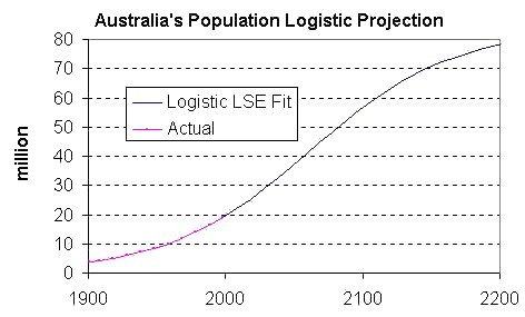
The logistic equation produces an S shaped curve as shown below.
For early years, the death rate is negligible (set d to zero in equation), and the curve is
indistinguishable from an exponential growth curve. But eventually
as the population increase, the death rate begins to have an
effect, flattening the growth curve...
A logistic curve can be fitted to Australia's population data
based on Source: Australian Demographic Statistics (3101.0);
Australian Demographic Trends (3102.0) - see www.abs.gov.au). This
exercise gave a mean-square error of 0.31 million, b = 0.0192 (ie. 1.9%), and d = 0.000231 and P0 = 3.63 million (ie
at 1900). The ratio b/d has the final
(asymptotic) value of 83 million.
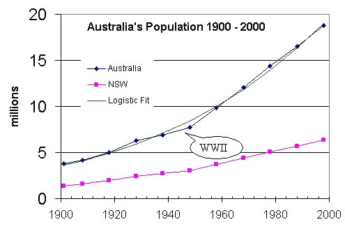
Least-square error fitting an exponential growth curve to the
same data gives a growth rate of 1.68% per annum, P0 =
3.77 million and a mean-square error of 0.35 million. So the
logistic equation is a better fit.
The goodness of fit can be seen in the graph below of
Australia's Population 1900 to 2000.
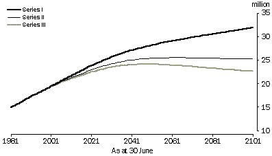
Here is the ABS's population projection, which is
considerably lower than the logistic estimate. The ABS is clearly
expecting future growth rates unlike the past.
If the underlying data is truly exponential, fitting a logistic
curve to it will give a d of 0.
Using It
Data can be fit to a logistic curve by using MS Excel's Solver tool, which uses a Generalized
Reduced Gradient Algorithm.
- Construct a spreadsheet with the actual data points.
- Set up cells for b , d, & P0 and a column for the P(t)
expression.
- Add a column showing the square error between P(t) and the
actual data points, and
- put a cell at the bottom of it giving the mean (average) square
error.
- Tick Assume non-negative in the solver options (disallows
negative d etc.,. - but you might
want to try some scenarios with this relaxed).
- Use Solver to minimize the mean square error cell by adjusting
b & d and P0 cells.
- For some problems, formulating the logistic equation with
P0 as 1 and using a time offset variable t0
instead may give better performance.
- Check solution is a global minima by choosing different initial
values (change singly and in pairs, by small and large amounts). If
you are really cute with Excel VBA, you could write a program to
randomly vary the initial values over a likely range.
Other Logistic Curves
See the following pages for applications of the logistic curve
to other situations:
First published 12th November 2000. Last 24th Jan 2017